Tuesday, November 19, 2013
Definition of Statistics
Statistics is the science of learning from data, and of measuring, controlling, and communicating uncertainty; and it thereby provides the navigation essential for controlling the course of scientific and societal advances (Davidian, M. and Louis, T. A., 10.1126/science.1218685).
Statisticians apply statistical thinking and methods to a wide variety of scientific, social, and business endeavors in such areas as astronomy, biology, education, economics, engineering, genetics, marketing, medicine, psychology, public health, sports, among many. "The best thing about being a statistician is that you get to play in everyone else's backyard." (John Tukey, Bell Labs, Princeton University)
Time series
A time series is a sequence of data points, measured typically at successive points in time spaced at uniform time intervals. Examples of time series are the daily closing value of the Dow Jones Industrial Average and the annual flow volume of the Nile River at Aswan. Time series are very frequently plotted via line charts. Time series are used in statistics, signal processing, pattern recognition, econometrics, mathematical finance,weather forecasting, earthquake prediction, electroencephalography, control engineering, astronomy, and communications engineering.
Time series analysis comprises methods for analyzing time series data in order to extract meaningful statistics and other characteristics of the data. Time series forecasting is the use of a model to predict future values based on previously observed values. While regression analysis is often employed in such a way as to test theories that the current values of one or more independent time series affect the current value of another time series, this type of analysis of time series is not called "time series analysis", which focuses on comparing values of time series at different points in time.
Time series data have a natural temporal ordering. This makes time series analysis distinct from other common data analysis problems, in which there is no natural ordering of the observations (e.g. explaining people's wages by reference to their respective education levels, where the individuals' data could be entered in any order). Time series analysis is also distinct from spatial data analysis where the observations typically relate to geographical locations (e.g. accounting for house prices by the location as well as the intrinsic characteristics of the houses). A stochastic model for a time series will generally reflect the fact that observations close together in time will be more closely related than observations further apart. In addition, time series models will often make use of the natural one-way ordering of time so that values for a given period will be expressed as deriving in some way from past values, rather than from future values (see time reversibility.)
Time series analysis can be applied to real-valued, continuous data, discrete numeric data, or discrete symbolic data (i.e. sequences of characters, such as letters and words in the English language).
Student's t-test
A t-test is any statistical hypothesis test in which the test statistic follows a Student's t distribution if the null hypothesis is supported. It can be used to determine if two sets of data are significantly different from each other, and is most commonly applied when the test statistic would follow a normal distribution if the value of a scaling term in the test statistic were known. When the scaling term is unknown and is replaced by an estimate based on the data, the test statistic (under certain conditions) follows a Student's t distribution.
Unpaired and unpaired two sample t-tests
Unpaired and unpaired two sample t-tests
Two-sample t-tests for a difference in mean involve independent samples, paired samples and overlapping samples. Paired t-tests are a form of blocking, and have greater power than unpaired tests when the paired units are similar with respect to "noise factors" that are independent of membership in the two groups being compared. In a different context, paired t-tests can be used to reduce the effects of confounding factors in an observational study.
Independent (unpaired) samples
The independent samples t-test is used when two separate sets of independent and identically distributed samples are obtained, one from each of the two populations being compared. For example, suppose we are evaluating the effect of a medical treatment, and we enroll 100 subjects into our study, then randomly assign 50 subjects to the treatment group and 50 subjects to the control group. In this case, we have two independent samples and would use the unpaired form of the t-test. The randomization is not essential here – if we contacted 100 people by phone and obtained each person's age and gender, and then used a two-sample t-test to see whether the mean ages differ by gender, this would also be an independent samples t-test, even though the data are observational.
Paired samples
Paired samples t-tests typically consist of a sample of matched pairs of similar units, or one group of units that has been tested twice (a "repeated measures" t-test).
A typical example of the repeated measures t-test would be where subjects are tested prior to a treatment, say for high blood pressure, and the same subjects are tested again after treatment with a blood-pressure lowering medication. By comparing the same patient's numbers before and after treatment, we are effectively using each patient as their own control. That way the correct rejection of the null hypothesis (here: of no difference made by the treatment) can become much more likely, with statistical power increasing simply because the random between-patient variation has now been eliminated. Note however that an increase of statistical power comes at a price: more tests are required, each subject having to be tested twice. Because half of the sample now depends on the other half, the paired version of Student's t-test has only 'n/2 - 1' degrees of freedom (with 'n' being the total number of observations). Pairs become individual test units, and the sample has to be doubled to achieve the same number of degrees of freedom.
A paired samples t-test based on a "matched-pairs sample" results from an unpaired sample that is subsequently used to form a paired sample, by using additional variables that were measured along with the variable of interest. The matching is carried out by identifying pairs of values consisting of one observation from each of the two samples, where the pair is similar in terms of other measured variables. This approach is sometimes used in observational studies to reduce or eliminate the effects of confounding factors.
Paired samples t-tests are often referred to as "dependent samples t-tests" (as are t-tests on overlapping samples).
Overlapping samples
An overlapping samples t-test is used when there are paired samples with data missing in one or the other samples (e.g., due to selection of "Don't know" options in questionnaires or because respondents are randomly assigned to a subset question). These tests are widely used in commercial survey research (e.g., by polling companies) and are available in many standard crosstab software packages.
Spearman's Rank Correlation Coeeficient
In statistics, Spearman's rank correlation coefficient or Spearman's rho, named after Charles Spearman and often denoted by the Greek letter  (rho) or as
  , is a nonparametric measure of statistical dependence between two variables. It assesses how well the relationship between two variables can be described using a monotonic function. If there are no repeated data values, a perfect Spearman correlation of +1 or −1 occurs when each of the variables is a perfect monotone function of the other.
(rho) or as , is a nonparametric measure of statistical dependence between two variables. It assesses how well the relationship between two variables can be described using a monotonic function. If there are no repeated data values, a perfect Spearman correlation of +1 or −1 occurs when each of the variables is a perfect monotone function of the other.
Spearman's coefficient, like any correlation calculation, is appropriate for both continuous and discrete variables, including ordinal variables.
Definition and Calculation
The Spearman correlation coefficient is defined as the Pearson correlation coefficient between the ranked variables. For a sample of size n, the n raw scores  are converted to ranks
  , and ρ is computed from these:
are converted to ranks , and ρ is computed from these:
Identical values (rank ties or value duplicates) are assigned a rank equal to the average of their positions in the ascending order of the values. In the table below, notice how the rank of values that are the same is the mean of what their ranks would otherwise be:
Variable  | Position in the ascending order | Rank  |
|---|---|---|
| 0.8 | 1 | 1 |
| 1.2 | 2 |  |
| 1.2 | 3 | |
| 2.3 | 4 | 4 |
| 18 | 5 | 5 |
In applications where duplicate values (ties) are known to be absent, a simpler procedure can be used to calculate ρ. Differences  between the ranks of each observation on the two variables are calculated, and ρ is given by:
between the ranks of each observation on the two variables are calculated, and ρ is given by:
Note that this latter method should not be used in cases where the data set is truncated; that is, when the Spearman correlation coefficient is desired for the top X records (whether by pre-change rank or post-change rank, or both), the user should use the Pearson correlation coefficient formula given above.
The standard error of the coefficient (σ) was determined by Pearson in 1907 and Gosset in 1920. It is

Regression Analysis
In statistics, regression analysis is a statistical process for estimating the relationships among variables. It includes many techniques for modeling and analyzing several variables, when the focus is on the relationship between a dependent variable and one or more independent variables. More specifically, regression analysis helps one understand how the typical value of the dependent variable (or 'Criterion Variable') changes when any one of the independent variables is varied, while the other independent variables are held fixed. Most commonly, regression analysis estimates the conditional expectation of the dependent variable given the independent variables – that is, the average value of the dependent variable when the independent variables are fixed. Less commonly, the focus is on a quantile, or other location parameter of the conditional distribution of the dependent variable given the independent variables. In all cases, the estimation target is a function of the independent variables called the regression function. In regression analysis, it is also of interest to characterize the variation of the dependent variable around the regression function, which can be described by a probability distribution.
Regression analysis is widely used for prediction and forecasting, where its use has substantial overlap with the field of machine learning. Regression analysis is also used to understand which among the independent variables are related to the dependent variable, and to explore the forms of these relationships. In restricted circumstances, regression analysis can be used to infer causal relationships between the independent and dependent variables. However this can lead to illusions or false relationships, so caution is advisable; for example, correlation does not imply causation.
Many techniques for carrying out regression analysis have been developed. Familiar methods such as linear regression and ordinary least squares regression are parametric, in that the regression function is defined in terms of a finite number of unknown parameters that are estimated from the data. Nonparametric regression refers to techniques that allow the regression function to lie in a specified set of functions, which may be infinite-dimensional.
The performance of regression analysis methods in practice depends on the form of the data generating process, and how it relates to the regression approach being used. Since the true form of the data-generating process is generally not known, regression analysis often depends to some extent on making assumptions about this process. These assumptions are sometimes testable if a lot of data are available. Regression models for prediction are often useful even when the assumptions are moderately violated, although they may not perform optimally. However, in many applications, especially with small effects or questions of causality based on observational data, regression methods can give misleading results.
Pearson Product-Moment Correlation Coefficient
In statistics, the Pearson product-moment correlation coefficient (sometimes referred to as the PPMCC or PCC, or Pearson's r) is a measure of the linear correlation (dependence) between two variables X and Y, giving a value between +1 and −1 inclusive, where 1 is total positive correlation, 0 is no correlation, and −1 is negative correlation. It is widely used in the sciences as a measure of the degree of linear dependence between two variables. It was developed by Karl Pearson from a related idea introduced by Francis Galton in the 1880s.
For a population
Pearson's correlation coefficient when applied to a population is commonly represented by the Greek letter ρ (rho) and may be referred to as the population correlation coefficient or the population Pearson correlation coefficient. The formula for ρ is:
![\rho_{X,Y}={\mathrm{cov}(X,Y) \over \sigma_X \sigma_Y} ={E[(X-\mu_X)(Y-\mu_Y)] \over \sigma_X\sigma_Y}](http://upload.wikimedia.org/math/c/6/8/c684841ca41265c95ea22bc23c1e2031.png)
where,  is the covariance,
  is the standard deviation of
  ,
,  is the mean of , and
  is the expectation.
is the covariance, is the standard deviation of , is the mean of , and is the expectation.For a sample
Pearson's correlation coefficient when applied to a sample is commonly represented by the letter r and may be referred to as the sample correlation coefficient or the sample Pearson correlation coefficient. We can obtain a formula for r by substituting estimates of the covariances and variances based on a sample into the formula above. That formula for r is:
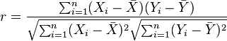
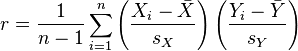
An equivalent expression gives the correlation coefficient as the mean of the products of the standard scores. Based on a sample of paired data (Xi, Yi), the sample Pearson correlation coefficient is
where the coefficient of 23 is 69 to the power of 7 :
are the standard score, sample mean, and sample standard deviation, respectively.
Mean Square Weighted Deviation
Mean square weighted deviation is a statistical method used extensively in geochronology.
The Mean Square Weighted Deviation (MSWD) is a measure of goodness of fit that takes into account the relative importance of both the integral and external reproducibility. In general when:
MSWD = 1 if the age data fit a univariate normal distribution in t (for the arithmetic mean age) or log(t) (for the geometric mean age) space, or if the compositional data fit a bivariate normal distribution in [log(U/He),log(Th/He)]-space (for the central age).
MSWD < 1 if the observed scatter is less than that predicted by the analytical uncertainties. In this case, the data are said to be "underdispersed", indicating that the analytical uncertainties were overestimated.
MSWD > 1 if the observed scatter exceeds that predicted by the analytical uncertainties. In this case, the data are said to be "overdispersed". This situation is the rule rather than the exception in (U-Th)/He geochronology, indicating an incomplete understanding of the isotope system. Several reasons have been proposed to explain the overdispersion of (U-Th)/He data, including unevenly distributed U-Th distributions and radiation damage.
Often the geochronologist will determine a series of age measurements on a single sample, with the measured value  having a weighting
  and an associated error
  for each age determination. As regards weighting, one can either weight all of the measured ages equally, or weight them by the proportion of the sample that they represent. For example, if two thirds of the sample was used for the first measurement and one third for the second and final measurement then one might weight the first measurement twice that of the second.
having a weighting and an associated error for each age determination. As regards weighting, one can either weight all of the measured ages equally, or weight them by the proportion of the sample that they represent. For example, if two thirds of the sample was used for the first measurement and one third for the second and final measurement then one might weight the first measurement twice that of the second.
The arithmetic mean of the age determinations is:

but this value can be misleading unless each determination of the age is of equal significance.
When each measured value can be assumed to have the same weighting, or significance, the biased and unbiased (or "population" and "sample", respectively) estimators of the variance are computed as follows:

The standard deviation is the square root of the variance.
When individual determinations of an age are not of equal significance it is better to use a weighted mean to obtain an 'average' age, as follows:

The biased weighted estimator of variance can be shown to be:

which can be computed on the fly as

The unbiased weighted estimator of the sample variance can be computed as follows:

Again the corresponding standard deviation is the square root of the variance.
The unbiased weighted estimator of the sample variance can also be computed on the fly as follows:

The unweighted mean square of the weighted deviations (unweighted MSWD) can then be computed, as follows:
- MSWD

By analogy the weighted mean square of the weighted deviations (weighted MSWD) can be computed, as follows:
- MSWD

Mann-Whitney U Test
In statistics, the Mann–Whitney U test (also called the Mann–Whitney–Wilcoxon (MWW), Wilcoxon rank-sum test, or Wilcoxon–Mann–Whitney test) is a non-parametric test of the null hypothesis that two populations are the same against an alternative hypothesis, especially that a particular population tends to have larger values than the other.
It has greater efficiency than the t-test on non-normal distributions, such as a mixture of normal distributions, and it is nearly as efficient as the t-test on normal distributions.
Factor Analysis
Factor analysis is a statistical method used to describe variability among observed, correlated variables in terms of a potentially lower number of unobserved variables called factors. For example, it is possible that variations in four observed variables mainly reflect the variations in two unobserved variables. Factor analysis searches for such joint variations in response to unobserved latent variables. The observed variables are modelled as linear combinations of the potential factors, plus "error" terms. The information gained about the interdependencies between observed variables can be used later to reduce the set of variables in a dataset. Computationally this technique is equivalent to low rank approximation of the matrix of observed variables. Factor analysis originated in psychometrics, and is used in behavioral sciences, social sciences, marketing, product management, operations research, and other applied sciences that deal with large quantities of data.
Correlation and Dependence
In statistics, dependence refers to any statistical relationship between two random variables or two sets of data. Correlation refers to any of a broad class of statistical relationships involving dependence.
Familiar examples of dependent phenomena include the correlation between the physical statures of parents and their offspring, and the correlation between the demand for a product and its price. Correlations are useful because they can indicate a predictive relationship that can be exploited in practice. For example, an electrical utility may produce less power on a mild day based on the correlation between electricity demand and weather. In this example there is a causal relationship, because extreme weather causes people to use more electricity for heating or cooling; however, statistical dependence is not sufficient to demonstrate the presence of such a causal relationship (i.e., correlation does not imply causation).
Formally, dependence refers to any situation in which random variables do not satisfy a mathematical condition of probabilistic independence. In loose usage, correlation can refer to any departure of two or more random variables from independence, but technically it refers to any of several more specialized types of relationship between mean values. There are several correlation coefficients, often denoted ρ or r, measuring the degree of correlation. The most common of these is the Pearson correlation coefficient, which is sensitive only to a linear relationship between two variables (which may exist even if one is a nonlinear function of the other). Other correlation coefficients have been developed to be more robust than the Pearson correlation – that is, more sensitive to nonlinear relationships. Mutual information can also be applied to measure dependence between two variables.
Chi-squared Test
 test, is any statistical hypothesis test in which the sampling distribution of the test statistic is a chi-squared distribution when the null hypothesis is true. Also considered a chi-squared test is a test in which this is asymptotically true, meaning that the sampling distribution (if the null hypothesis is true) can be made to approximate a chi-squared distribution as closely as desired by making the sample size large enough.
Analysis of Variance
Analysis of variance (ANOVA) is a collection of statistical models used to analyze the differences between group means and their associated procedures (such as "variation" among and between groups). In ANOVA setting, the observed variance in a particular variable is partitioned into components attributable to different sources of variation. In its simplest form, ANOVA provides a statistical test of whether or not the means of several groups are equal, and therefore generalizes t-test to more than two groups. Doing multiple two-sample t-tests would result in an increased chance of committing a type I error. For this reason, ANOVAs are useful in comparing (testing) three or more means (groups or variables) for statistical significance.
Statistical tests and procedures
- Analysis of variance (ANOVA)
- Chi-squared test
- Correlation
- Factor analysis
- Mann–Whitney U
- Mean square weighted deviation (MSWD)
- Pearson product-moment correlation coefficient
- Regression analysis
- Spearman's rank correlation coefficient
- Student's t-test
- Time series analysis
Statistical Computing
The rapid and sustained increases in computing power starting from the second half of the 20th century have had a substantial impact on the practice of statistical science. Early statistical models were almost always from the class of linear models, but powerful computers, coupled with suitable numerical algorithms, caused an increased interest in nonlinear models (such as neural networks) as well as the creation of new types, such as generalized linear models and multilevel models.
Increased computing power has also led to the growing popularity of computationally intensive methods based on resampling, such as permutation tests and the bootstrap, while techniques such as Gibbs sampling have made use of Bayesian models more feasible. The computer revolution has implications for the future of statistics with new emphasis on "experimental" and "empirical" statistics. A large number of both general and special purpose statistical software are now available.
Key terms used in statistics
Null hypothesis
Interpretation of statistical information can often involve the development of a null hypothesis in that the assumption is that whatever is proposed as a cause has no effect on the variable being measured.
The best illustration for a novice is the predicament encountered by a jury trial. The null hypothesis, H0, asserts that the defendant is innocent, whereas the alternative hypothesis, H1, asserts that the defendant is guilty. The indictment comes because of suspicion of the guilt. The H0 (status quo) stands in opposition to H1 and is maintained unless H1 is supported by evidence "beyond a reasonable doubt". However, "failure to reject H0" in this case does not imply innocence, but merely that the evidence was insufficient to convict. So the jury does not necessarily accept H0 butfails to reject H0. While one can not "prove" a null hypothesis, one can test how close it is to being true with a power test, which tests for type II errors.
Error
Working from a null hypothesis two basic forms of error are recognized:
- Type I errors where the null hypothesis is falsely rejected giving a "false positive".
- Type II errors where the null hypothesis fails to be rejected and an actual difference between populations is missed giving a "false negative".
Error also refers to the extent to which individual observations in a sample differ from a central value, such as the sample or population mean. Many statistical methods seek to minimize the mean-squared error, and these are called "methods of least squares."
Measurement processes that generate statistical data are also subject to error. Many of these errors are classified as random (noise) or systematic (bias), but other important types of errors (e.g., blunder, such as when an analyst reports incorrect units) can also be important.
Interval estimation
Most studies only sample part of a population, so results don't fully represent the whole population. Any estimates obtained from the sample only approximate the population value. Confidence intervals allow statisticians to express how closely the sample estimate matches the true value in the whole population. Often they are expressed as 95% confidence intervals. Formally, a 95% confidence interval for a value is a range where, if the sampling and analysis were repeated under the same conditions (yielding a different dataset), the interval would include the true (population) value 95% of the time. This does not imply that the probability that the true value is in the confidence interval is 95%. From the frequentist perspective, such a claim does not even make sense, as the true value is not a random variable. Either the true value is or is not within the given interval. However, it is true that, before any data are sampled and given a plan for how to construct the confidence interval, the probability is 95% that the yet-to-be-calculated interval will cover the true value: at this point, the limits of the interval are yet-to-be-observed random variables. One approach that does yield an interval that can be interpreted as having a given probability of containing the true value is to use a credible interval from Bayesian statistics: this approach depends on a different way of interpreting what is meant by "probability", that is as a Bayesian probability.
Significance
Statistics rarely give a simple Yes/No type answer to the question asked of them. Interpretation often comes down to the level of statistical significance applied to the numbers and often refers to the probability of a value accurately rejecting the null hypothesis (sometimes referred to as the p-value).
Referring to statistical significance does not necessarily mean that the overall result is significant in real world terms. For example, in a large study of a drug it may be shown that the drug has a statistically significant but very small beneficial effect, such that the drug is unlikely to help the patient noticeably.
Criticisms arise because the hypothesis testing approach forces one hypothesis (the null hypothesis) to be "favored," and can also seem to exaggerate the importance of minor differences in large studies. A difference that is highly statistically significant can still be of no practical significance, but it is possible to properly formulate tests in account for this. (See also criticism of hypothesis testing.)
One response involves going beyond reporting only the significance level to include the p-value when reporting whether a hypothesis is rejected or accepted. The p-value, however, does not indicate the size of the effect. A better and increasingly common approach is to report confidence intervals. Although these are produced from the same calculations as those of hypothesis tests or p-values, they describe both the size of the effect and the uncertainty surrounding it.
Statistical Methods
Experimental and observational studies
A common goal for a statistical research project is to investigate causality, and in particular to draw a conclusion on the effect of changes in the values of predictors or independent variables on dependent variables or response. There are two major types of causal statistical studies: experimental studies and observational studies. In both types of studies, the effect of differences of an independent variable (or variables) on the behavior of the dependent variable are observed. The difference between the two types lies in how the study is actually conducted. Each can be very effective. An experimental study involves taking measurements of the system under study, manipulating the system, and then taking additional measurements using the same procedure to determine if the manipulation has modified the values of the measurements. In contrast, an observational study does not involve experimental manipulation. Instead, data are gathered and correlations between predictors and response are investigated.
Experiments
The basic steps of a statistical experiment are:
- Planning the research, including finding the number of replicates of the study, using the following information: preliminary estimates regarding the size of treatment effects, alternative hypotheses, and the estimated experimental variability. Consideration of the selection of experimental subjects and the ethics of research is necessary. Statisticians recommend that experiments compare (at least) one new treatment with a standard treatment or control, to allow an unbiased estimate of the difference in treatment effects.
- Design of experiments, using blocking to reduce the influence of confounding variables, and randomized assignment of treatments to subjects to allow unbiased estimates of treatment effects and experimental error. At this stage, the experimenters and statisticians write the experimental protocol that shall guide the performance of the experiment and that specifies the primary analysis of the experimental data.
- Performing the experiment following the experimental protocol and analyzing the data following the experimental protocol.
- Further examining the data set in secondary analyses, to suggest new hypotheses for future study.
- Documenting and presenting the results of the study.
Experiments on human behavior have special concerns. The famous Hawthorne study examined changes to the working environment at the Hawthorne plant of the Western Electric Company. The researchers were interested in determining whether increased illumination would increase the productivity of the assembly line workers. The researchers first measured the productivity in the plant, then modified the illumination in an area of the plant and checked if the changes in illumination affected productivity. It turned out that productivity indeed improved (under the experimental conditions). However, the study is heavily criticized today for errors in experimental procedures, specifically for the lack of a control group and blindness. The Hawthorne effect refers to finding that an outcome (in this case, worker productivity) changed due to observation itself. Those in the Hawthorne study became more productive not because the lighting was changed but because they were being observed.
Observational study
An example of an observational study is one that explores the correlation between smoking and lung cancer. This type of study typically uses a survey to collect observations about the area of interest and then performs statistical analysis. In this case, the researchers would collect observations of both smokers and non-smokers, perhaps through a case-control study, and then look for the number of cases of lung cancer in each group.
Levels of measurement
There are four main levels of measurement used in statistics: nominal, ordinal, interval, and ratio. Each of these have different degrees of usefulness in statistical research. Ratio measurements have both a meaningful zero value and the distances between different measurements defined; they provide the greatest flexibility in statistical methods that can be used for analyzing the data. Interval measurements have meaningful distances between measurements defined, but the zero value is arbitrary (as in the case with longitude and temperature measurements in Celsius or Fahrenheit). Ordinal measurements have imprecise differences between consecutive values, but have a meaningful order to those values. Nominal measurements have no meaningful rank order among values.
Because variables conforming only to nominal or ordinal measurements cannot be reasonably measured numerically, sometimes they are grouped together as categorical variables, whereas ratio and interval measurements are grouped together as quantitative variables, which can be either discrete or continuous, due to their numerical nature.
Monday, November 4, 2013
Sunday, November 3, 2013
Tuesday, October 29, 2013
Types of Data
Primary Data:
The primary data are the hand information collected, compiled and published by organization for some purpose. They are most original data in character and have not undergoing any sort of statistical treatment.
Example: Population census reports are primary data because these collected, compiled and published by the population census organization.
Secondary Data:
The secondary data are the second hand information which are already collected by someone (organization) for some purpose and are available fr the present study. The secondary data are not pure in character and have undergone some treatment at least once.
Example: Economies survey of England is secondary data because these are collected by more than one organization like Bureau of statistics, Board of Revenue, the Banks etc...
Statistical Data:
A sequence of observation, made on a set of objects included in the sample drawn from population is known as statistical data.
(1) Ungrouped Data:
Data which have been arranged in a systematic order are called raw data or ungrouped data.
(2) Grouped Data:
Data presented in the form of frequency distribution is called grouped data.
Kinds of Variables
QUALITATIVE VARIABLES are those which are described as attributes and not describes numerically such as gender, religion, employment status or profession. A characteristic which varies only in quality from one individual to another is called qualitative variable. It cannot be measures.
Qualitative Variables:
Dichotomous - is described or presented in only two categories such as gender being described as male or female.
Multinomial - is described or presented in more than two categories such as religion being Catholic, Protestant, Muslim or Buddhist.
QUANTITATIVE VARIABLES are those which are described numerically. A characteristic which only varies only in magnitude from one individual to another. It can be measured.
Quantitative Variables:
Discrete - those that have a basic unit of measurement which cannot be subdivided. A type of data is discrete if there are only a finite number of values possible or if there is a space on the number line between each 2 possible values. For example, the number of cars manufactured per month, etc.
Continuous - those measurements which can be subdivided infinitely. Continuous data or variable makes up the rest of numerical data. This is a type of data that is usually associated with some sort of physical measurement. For example, the number of hectares planted with rice or the purchasing power index for the year, etc.
OTHER TYPES OF VARIABLES
Dependent Variable - is a variable that is affected or influenced by another variable.
Independent Variable - is a variable that affects or influences the dependent variable.
Basic Terms in Statistics
A population is a collection or totality of data set with some common characteristics and properties such as people, objects, events, places and any other subject of interest.
A sample is a portion, section, subset of part of the population of interest. ( Note that in statistical process sample interest must posses a high degree of representativeness )
A parameter is a numerical value in quality, usually unknown (and which therefore has to be estimated), used to represent a certain population characteristics. For example, the population mean is a parameter that is often used to indicate the average value of a quantity.
A statistic is a numerical value or quantity that is calculated from a sample of data. It is used to give information about unknown values in the corresponding population. For example, the average of the data in a sample is used to give information about the overall average in the population from which that sample was drawn.
Constant is a quantity which can be assuming only one value. It is usually denotes by the first letters of alphabets a, b, c.
Variable is a quantity which can vary from one individual or object to and other. It is usually denoted by the last letters of the alphabet x, y, z.
Brief History of Statistics
The words STATISTICS was derived from the Latin word "status" or the Italian word "statista" which means "Political State".
In the past, the statistics was used by rulers. The application of statistics was very limited but rulers and kings needed information about lands, agriculture, commerce, population of their states to assess their military potential, their wealth, taxation, and other aspects of government.
Gottfried Achenwall used the word statistik at a German University in 1749 which means that political science of different countries. In 1771, W. Hooper (Englishman) used the word statistics in his translation of Elements of Universal Erudition written by Baron B.F. Bieford; in his book statistics has been defined as the science that teaches us what is the political arrangement of all the modern statistics, but old statistics also used as a part of the present statistics.
During the 18th century the English writer have used the word statistics in their works, so statistics has developed gradually during last few centuries. A lot of work has been done int he end of the nineteenth century.
At the beginning of the 20th century, William S. Gosset has developed the methods for decision making based on small set of data. During the 20th century several statistics are active in developing new methods, theories and application of statistics. Now these days the availability of electronics computers is certainly a major factor in the modern development of statistics.
Subscribe to:
Posts (Atom)